Analysis and removal of serial correlations in time series, and analysis of the impact of an external disturbance ("intervention") at a particular point in time. Assumes stationary time series, except for a single intervention. Requires one column of equally spaced data.
This powerful but somewhat complicated module implements maximum-likelihood ARMA analysis, and a minimal version of Box-Jenkins intervention analysis (e.g. for investigating how a climate change might impact biodiversity).
By default, a simple ARMA analysis without interventions is computed. The user selects the number of AR (autoregressive) and MA (moving-average) terms to include in the ARMA difference equation. The log-likelihood and Akaike information criterion are given. Select the numbers of terms that minimize the Akaike criterion, but be aware that AR terms are more "powerful" than MA terms. Two AR terms can model a periodicity, for example.
The main aim of ARMA analysis is to remove serial correlations, which otherwise cause problems for model fitting and statistics. The residual should be inspected for signs of autocorrelation, e.g. by copying the residual from the numerical output window back to the spreadsheet and using the autocorrelation module. Note that for many paleontological data sets with sparse data and confounding effects, proper ARMA analysis (and therefore intervention analysis) will be impossible.
The program is based on the likelihood algorithm of Melard (1984), combined with nonlinear multivariate optimization using simplex search.
Intervention analysis
Intervention analysis proceeds as follows. First, carry out ARMA analysis on only the samples preceding the intervention, by typing the last pre-intervention sample number in the "last samp" box. It is also possible to run the ARMA analysis only on the samples following the intervention, by typing the first post-intervention sample in the "first samp" box, but this is not recommended because of the post-intervention disturbance. Also tick the "Intervention" box to see the optimized intervention model.
The analysis follows Box and Tiao (1975) in assuming an "indicator function" u(i) that is either a unit step or a unit pulse, as selected by the user. The indicator function is transformed by an AR(1) process with a parameter delta, and then scaled by a magnitude (note that the magnitude given by PAST is the coefficient on the transformed indicator function: first do y(i)=delta*y(i-1)+u(i), then scale y by the magnitude). The algorithm is based on ARMA transformation of the complete sequence, then a corresponding ARMA transformation of y, and finally linear regression to find the magnitude. The parameter delta is optimized by exhaustive search over [0,1].
For small impacts in noisy data, delta may end up on a sub-optimum. Try both the step and pulse options, and see what gives smallest standard error on the magnitude. Also, inspect the "delta optimization" data, where standard error of the estimate is plotted as a function of delta, to see if the optimized value may be unstable.
The Box-Jenkins model can model changes that are abrupt and permanent (step function with delta=0, or pulse with delta=1), abrupt and non-permanent (pulse with delta<1), or gradual and permanent (step with delta<0).
Be careful with the standard error on the magnitude - it will often be underestimated, especially if the ARMA model does not fit well. For this reason, a p value is deliberately not computed (Murtaugh 2002).
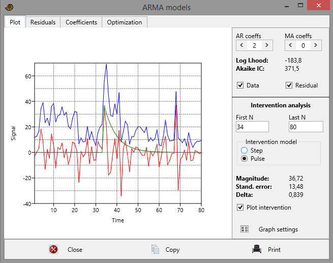
The example data set (blue curve) is Sepkoski’s curve for percent extinction rate on genus level since the Silurian, interpolated to even spacing at ca. 5.5 million years. The largest peak is the PermianTriassic boundary extinction. The user has specified an ARMA(2,0) model. The residual is plotted in red. The user has specified that the ARMA parameters should be computed for the points before the P-T extinction at time slot 34, and a pulse-type intervention. The analysis seems to indicate a large time constant (delta) for the intervention, with an effect lasting into the Jurassic.
References
Box, G.E.P. & G.C. Tiao. 1975. Intervention analysis with applications to economic and environental problems. Journal of the American Statistical Association 70:70-79.
Melard, G. 1984. A fast algorithm for the exact likelihood of autoregressive-moving average models. Applied Statistics 33:104-114.
Murtaugh, P.A. 2002. On rejection rates of paired intervention analysis. Ecology 83:1752-1761.