This module suggests positions of abrupt change (changepoints) in a time series, with constant values between the changepoints. The input data should be a single column with a series of numbers, or multiple columns with multivariate data collected at the same points in time or stratigraphy. An example application is the detection of breaks in multivariate geochemical data through a sediment core. The module implements the method described by Gallagher et al. (2011).
The algorithm is Bayesian, “transdimensional” Markov chain Monte Carlo (MCMC). It produces not a single set of model parameters, but a large number as samples (“simulations”) from the probability distribution.
For multiple-column data sets, note that each column is weighted equally, as mean and standard deviation are automatically normalized away prior to modeling.
Max chpoints: The maximal number of changepoints. This can often be left at the default, 10, unless you want to allow a larger or enforce a smaller number of changepoints. After analysis, the actual average number of changepoints (across simulations) is reported.
Simulations: The number of MCMC iterations, default 100 000. This includes the so-called burn-in, which is the initial number of simulations before the algorithm hopefully converges and data start to be collected. The number of burn-in iterations is fixed at 20 000. The “History” curve (see below) should be inspected to see if the number of simulations should be increased. For noisy data, it may be necessary to increase the number of simulations to a million or more, giving long computation times.
Changepoints plot: Shows a histogram of the positions of changepoints across all simulations.
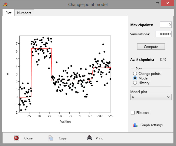
Model plot: Shows the average changepoint model as a red curve superimposed on the given data points. If most simulations agree on the changepoint positions, this will be a step-like curve (i.e. constant between changepoints). Variance (i.e. uncertainty) in changepoint positions will give a more rounded appearance. For multivariate data, you can select the plotted variable in the drop-down menu.
History: Shows the model log likelihood as a function of iteration number. Ideally, this curve should start at some large negative value, and quickly increase to a relatively stable value, varying as unstructured noise around a mean. The end of the burn-in is shown as a vertical line. If the log likelihood does not seem to stabilize, the number of simulations may have to be increased.
Missing values are treated by linear interpolation before the analysis.
Reference
Gallagher, K., Bodin, T., Sambridge, M., Weiss, D., Kylander, M., Large, D. 2011. Inference of abrupt changes in noisy geochemical records using transdimensional changepoint models. Earth and Planetary Science Letters 311:182-194.