Principal components analysis (PCA) finds hypothetical variables (components) accounting for as much as possible of the variance in your multivariate data (e.g. Legendre & Legendre 1998). These new variables are linear combinations of the original variables. PCA may be used for reduction of the data set to only two variables (the two first components), for plotting purposes. One might also hypothesize that the most important components are correlated with other underlying variables. For morphometric data, this might be size, while for ecological data it might be a physical gradient (e.g. temperature or depth).
The input data is a matrix of multivariate data, with items in rows and variates in columns.
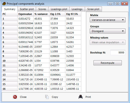
The PCA routine finds the eigenvalues and eigenvectors of the variance-covariance matrix or the correlation matrix, with the SVD algorithm. Use variance-covariance if all variables are measured in the same units (e.g. centimetres). Use correlation (normalized var-covar) if the variables are measured in different units; this implies normalizing all variables using division by their standard deviations. The eigenvalues give a measure of the variance accounted for by the corresponding eigenvectors (components). The percentages of variance accounted for by these components are also given. If most of the variance is accounted for by the first one or two components, you have scored a success, but if the variance is spread more or less evenly among the components, the PCA has in a sense not been very successful.
In the example below (landmarks from gorilla skulls), component 1 is strong, explaining 45.9% of variance. The bootstrapped confidence intervals are not shown unless the ‘Bootstrap N’ value is non-zero.
Groups
If groups are specified with a group column, the PCA can optionally be carried out within-group or between-group. In within-group PCA, the average within each group is subtracted prior to eigenanalysis, essentially removing the differences between groups. In between-group PCA, the eigenanalysis is carried out on the group means (i.e. the items analysed are the groups, not the rows). For both within-group and between-group PCA, the PCA scores are computed using vector products with the original data.
Supplementary variables
It is possible to include one or more initial columns containing additional supplementary variables for the analysis. These variables are not included in the ordination. The correlation coefficients between each supplementary variable and the PCA scores are presented as vectors from the origin (triplot). The lengths of the vectors are arbitrarily scaled to make a readable plot, so only their directions and relative lengths should be considered.
Bootstrapping
Row-wise bootstrapping is carried out if a positive number of bootstrap replicates (e.g. 1000) is given in the 'Bootstrap N' box. The bootstrapped components are re-ordered and reversed according to Peres-Neto et al. (2003) to increase correspondence with the original axes. 95% bootstrapped confidence intervals are given for the eigenvalues.
Scree plot
The 'Scree plot' (simple plot of eigenvalues) may also indicate the number of significant components. After this curve starts to flatten out, the components may be regarded as insignificant. 95% confidence intervals are shown if bootstrapping has been carried out. The eigenvalues expected under a random model (Broken Stick) are optionally plotted - eigenvalues under this curve may represent non-significant components (Jackson 1993).
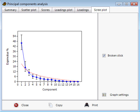
In the gorilla example above, the eigenvalues for the 16 components (blue line) lie above the broken stick values (red dashed line) for the first two components, although the broken stick is inside the 95% confidence interval for the second component.
Scatter plot
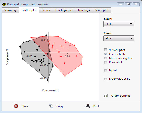
The scatter plot shows all data points (rows) plotted in the coordinate system given by two of the components. If you have groups, they can be emphasized with concentration ellipses or convex hulls. The Minimal Spanning Tree is the shortest possible set of lines connecting all points. This may be used as a visual aid in grouping close points. The MST is based on an Euclidean distance measure of the original data points, and is most meaningful when all variables use the same unit. The 'Biplot' option shows a projection of the original axes (variables) onto the scattergram. This is another visualisation of the PCA loadings (coefficients) - see below.
If the "Eigenval scale" is ticked, the scores and eigenvectors will be scaled to give the correlation biplot of Legendre & Legendre (1998). If not ticked, the scores are not scaled, while the biplot eigenvectors are normalized to equal length (but not to unity, for graphical reasons) - this is the distance biplot.
Loadings
The loadings plot shows to what degree your different original variables (given in the original order along the x axis) enter into the different components (as chosen in the radio button panel). These component loadings are important when you try to interpret the 'meaning' of the components. The 'Coefficients' option gives the PC coefficients, while 'Correlation' gives the correlation between a variable and the PC scores. If bootstrapping has been carried out, 95% confidence intervals are shown (only for the Coefficients option).
Sphericity tests
Bartlett's sphericity test (Bartlett 1951) tests the null hypothesis that the points are sampled from a spherical distribution. If so, PCA will not be able to provide a useful reduction of dimensionality. The p value from this test should ideally be less than 0.05 (significant departure from sphericity). The test is usually used for PCA on the correlation matrix.
Past also provides a Bartlett's sphericity test for PCA on the var-covar matrix, following Bartlett (1951). However, this test is not in common use, and its properties are not quite clear. It assumes equal variances in the variables. Use with caution.
The Kaiser-Meyer-Olkin (KMO) measure (Kaiser 1970), also known as Measure of Sampling Adequacy (MSA), is only supported for PCA on the correlation matrix.
KMO < 0.5 is reported as "unacceptable"; 0.5 < KMO < 0.7 is reported as “mediocre”; 0.7 < KMO <0.8 is “good”; 0.8 < KMO < 1 is “excellent”.
Missing values
Missing data can be handled by one of two methods:
- Mean value imputation: Missing values are replaced by their column average. Not recommended.
- Iterative imputation: Missing values are inititally replaced by their column average. An initial PCA run is then used to compute regression values for the missing data. The procedure is iterated until convergence. This is usually the preferred method, but can cause some overestimation of the strength of the components (see Ilin & Raiko 2010).
References
Bartlett, M.S. 1951. The effect of standardization on a chi-2 approximation in factor analysis. Biometrika 38:337-344.
Ilin, A. & T. Raiko. 2010. Practical approaches to Principal Component Analysis in the presence of missing values. Journal of Machine Learning Research 11:1957-2000.
Jackson, D.A. 1993. Stopping rules in principal components analysis: a comparison of heuristical and statistical approaches. Ecology 74:2204-2214.
Kaiser, H.F. 1970. A second generation little jiffy. Psychometrika 35:401-415.
Legendre, P. & L. Legendre. 1998. Numerical Ecology, 2nd English ed. Elsevier, 853 pp.
Peres-Neto, P.R., D.A. Jackson & K.M. Somers. 2003. Giving meaningful interpretation to ordination axes: assessing loading significance in principal component analysis. Ecology 84:2347-2363.